Computing, Math and Beauty

Fixpoints are values that a function maps to themselves, i.e., $f(x) = x$. Note that the domain and range of such functions have to overlap. At the very least the domain has to be restricted to the range. For example, if $f(x) = x^2$ then there are two fixpoints: $\{0, 1\}$. That's it, there is nothing fancy about it. The beauty is its simplicity. A lot of algorithms look much clearer if we look at them through the lens of fixpoints. This post is about looking at some algorithms that feel very foggy to think about but become very very clear once we think through this lens.

Banach Fixpoint Theorem

Before we dig deeper into the specific algorithms, we are going to look at a way to find fixpoints for a specific set of functions called Contractions. Contractions are functions whose values get closer in some notion of distance. For example, In $f(x) = \frac{x}{2}$, $f(1) = 1/2$ and $f(2) = 1$, the distance between the results is half of the distance between the arguments ($|1 - 2| > |\frac{1}{2} - 1|$). This doesn't necessarily have to be absolute difference. It can be any distance metric that satisfies Triangle Inequality. In fact a substantial number of functions on abstract structures or data types could be thought of as contractions with some notion of distance.

Banach proved in his Contraction Mapping Theorem that contractions admit at least one fixpoint. And the beautiful part is we can even chase down such fixpoints. Take any point in the domain, let's say $x$ and find $f(x)$, $f(f(x))$, $f(f(f(x)))$ it would eventually converge to $f(y) = y$. The intuition is very simple, Banach just showed that all roads lead to Rome. And Rome is a fixpoint.

Banach showed contraction maps have a fixpoint. And we can reach it by just repeatedly applying the function on any point.

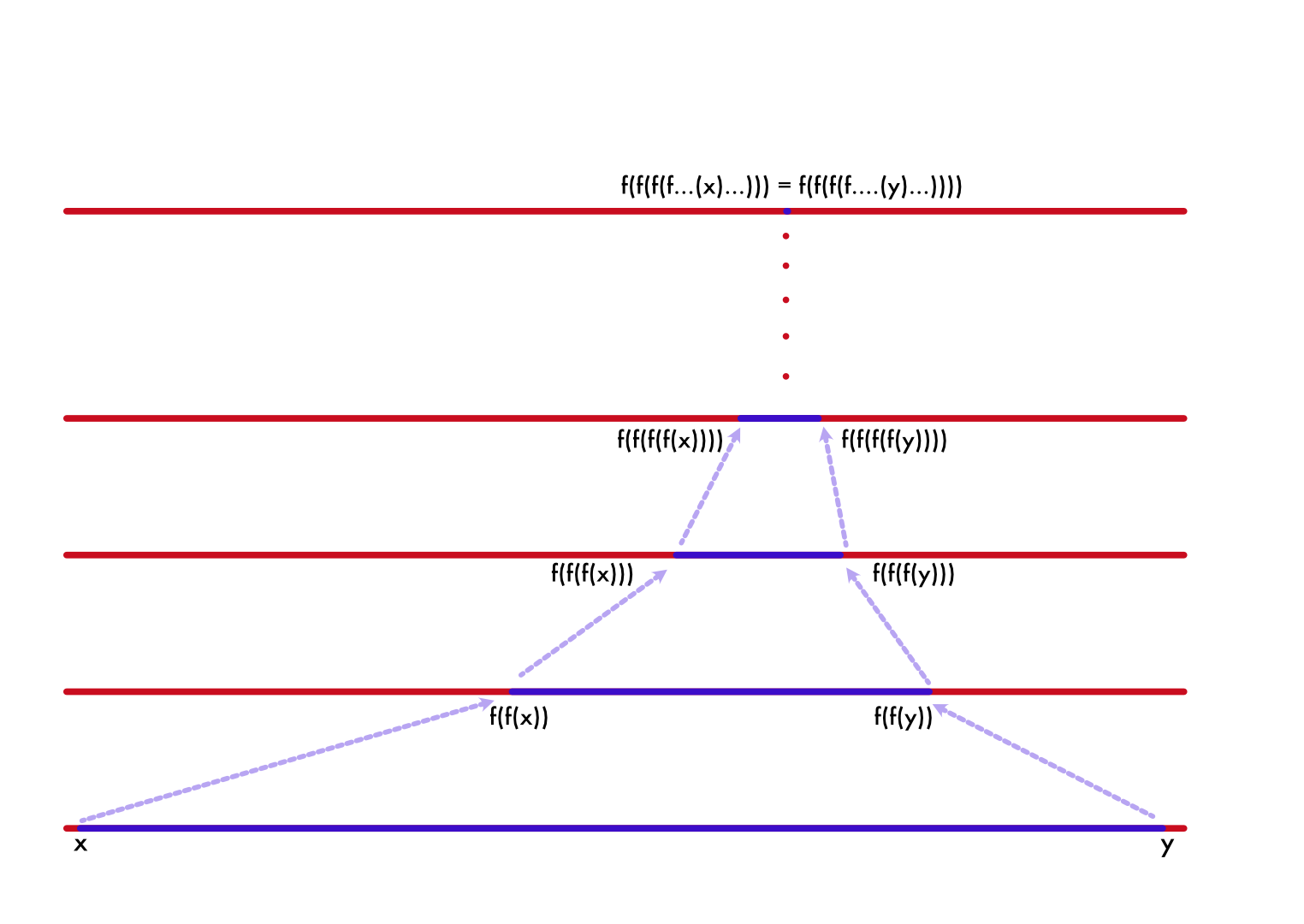
That gives us an algorithm to find fixpoints of arbitrary function (assuming contraction, which a substantial number of functions are, if we restrict the domain). Just take an arbitrary value in range/domain and reapply it until the function produces value very close to the argument or over a certain number of iterations, when the initial point is not in the contraction domain.

Page rank

In 1999, Larry Page and Sergey Brin were trying to solve the problem of ranking webpages for their search engine BackRub (which eventually became Google). They wanted to rank pages based on how many links each page got from other pages. But just weighing based on number of links a page got would lead to gaming the system. So they wanted to weigh the links based on the source's rank. This kind of got recursive because the source's rank depends on the rank of all the pages including the destination's rank (assuming that page had a link to the source). It suddenly feels intractable where do we start, how do we find ranks for all pages if they all depend on their own rank.

To illustrate this, let's assume we have pages $A, B, C, D, E$ and each page has links to other pages like this.

Hypothetical example of web with pages A, B, C, D & E with links between each other. We would like to find the rank/score for each of the page's importance just from their link structure and nothing else. This has nothing to do with relevance for the user query FYI.

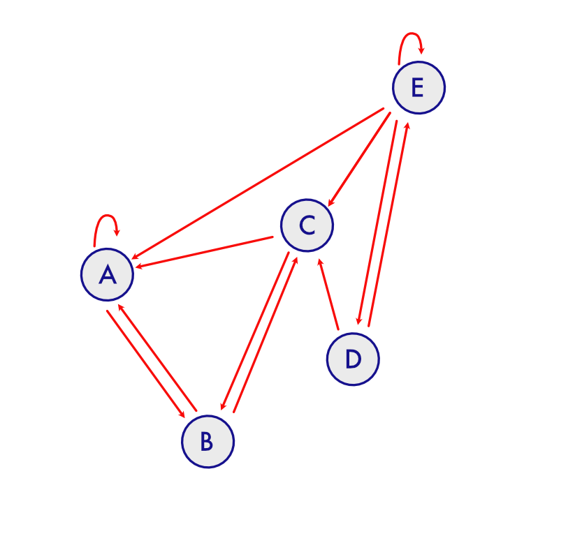
This could be represented in matrix form with number of outgoing (for column and incoming for row), each of $A, B, C, D, E$ if we assign indices $0, 1, 2, 3, 4$ respectively for them.

Let's rephrase the problem, suppose a person randomly starts in one of the pages, and he (uniformly) randomly clicks on one of the links on the page. What's the probability that after infinitely many steps, he would be on a particular page? And that is the probability Brin and Page wanted to assign as rank of the page. Given an array (vector) of probabilities that a person is currently in each of the pages and a function $f$ that finds the probabilities that a person would be in each of the pages in one round of clicking, they wanted to find $f(f(f(....)))$ of such a function. Which means if such a vector exists, let's call it $x = f(f(f(....)))$ then applying $f$ one more time wouldn't make a difference. We call that a stable state and if you haven't already figured it out it's a fixed point $x = f(x)$.

The only problem that remains is we need such an $f$. Assuming each link in page has equal chance of getting clicked. The probability of a person reaching page $x$ from $y$ is $\frac{\text{number of links to page x from y}}{\text{total number of links in y}}$. If we normalize the matrix by the sum of each column, then each cell represents the probability of reaching page $i$ from $j$ ($P(i|j)$).

We basically have $f$, we take the vector of probabilities and multiply it on the left with the above matrix. There are few practical issues with the above matrix, like what happens to islands and starting vector not reaching all the pages. Both of them are practically mitigated by assigning small probability to move to any page from any page. Sort of like a person typing in a URL at random or clicking on a link sent to him over email for example. Once we have that, it will reach stable state no matter where we start (due to spectral property that it will settle into dominant eigen vector, we can talk about that in another blog post maybe.) Hence the algorithm is like this.

                    
# This surprisingly converges very fast
# Even for large matrices, it would need < 100 iterations
# Depends on ratio of first and second largest eigen values
MAX_ITERATIONS = 10 
EPSILON = 0.001
def page_rank(links):
    epsilon_added = links + np.ones_like(links) * 0.001
    normalized = epsilon_added / np.sum(epsilon_added, axis = 0)
    num_iterations = 0
    rank = np.random.rand(links.shape[0])
    while num_iterations < MAX_ITERATIONS:
        next = normalized @ rank
        convergence = np.abs(rank.T @ next) < EPSILON
        num_iterations += 1
        rank = next / np.linalg.norm(next)
        if convergence:
            break
    return rank
                
            

Game equilibrium - Nash and others

Suppose there is a duopoly of companies (A, B) which produces soap. Since the demand is capped, as there is no reason for consumers to buy more fast moving goods than necessary, their profitability depends not just on how much each company is producing but also on how much their competitor is producing. Let's say they produce $a$ and $b$ quantities, let's assume the price that either of them could place is $P(a, b) = 2 - (a + b)$. Now how much "should" each of them produce, provided they are rational. We could analytically find the solution for this particular problem, however trying to find/reason about a general solution is definitely more enlightening, journey is worth more than the endpoint.

Given a fixed $b$, $a$ should be $\underset{a}{\operatorname{argmax}}{P(a, b) * a} $ ($argmax$ means argument which produces maximum value for a given target function). And we can similarly define a strategy for $b$ too. This is called Nash equilibrium for this game/decision. Once we find such a $a$ and $b$ there is no way they are going to be more profitable from diverging from that (duh, it's max). Hence it's an equilibrium.

This follows the exact same conundrum that we had before too, my decision depends on someone's decision whose decision depends on mine, except this time it's not a single function, we have 2 functions. One optimizes for $a$ and other optimizes for $b$, let's call them $f_a$ and $f_b$. To change it into familiar form, we just apply them one after another like

                    
def g(a, b):
    a_next = f_a(a, b)
    b_next = f_b(a_next, b)
    (a_next, b_next)
    
                

Now we just need to find the fixpoint for this problem. We could start with any quantity for $a$ and $b$ and find the solution. This however finds a non-integer quantity and we can round down to find a very good solution for this. However, if one of them rounds down and the other should round up, assuming rationality of players and hence not really an equilibrium.

                
LEARNING_RATE = 0.1

def price(a, b):
    return 2 - (a + b)

# gradient with respect to first variable it's symmetric, 
# we can swap arguments and get for other one.
def gradient(a, b):
    return 2 - 2 * a - b

def f_a(a, b):
    return a + LEARNING_RATE * gradient(a, b)

def f_b(a, b):
    return b + LEARNING_RATE * gradient(b, a)

MAX_ITERATIONS = 100

def equilibrium():
    num_iterations = 0
    a = 1
    b = 1
    while num_iterations < MAX_ITERATIONS:
        # No negatives.
        a_next = max(0.001, f_a(a, b))
        b_next = max(0.001, f_b(a_next, b)) 
        num_iterations += 1
        if np.abs(a - a_next) < EPSILON and np.abs(b - b_next) < EPSILON:
            break
        a = a_next
        b = b_next
    return a_next, b_next
                
            

This could very well be solved analytically, we just need to equate each of their gradient to 0 and find the solution. But again the idea is not a solution but a framework to think about problems like this. For example, our framework could help us get to Quantal equilibrium (replace max with softmax function, to elucidate fallible rationality) or Security solution (where the opponent is out there to get you even at the cost of his own utility). However, analytical solutions have to be worked out from scratch for each of them. This circular dependency shows up a lot in another interesting field of Reinforcement learning. Here is the problem which is a bit more complicated than the above which is stated in Reinforcement learning book by Sutton and Barto. The problem goes like this, a player lives in the $5 \times 5$ grid world. The player can move one step up/down/left/right which costs $-1$ units. There is a wormhole at $0,1$ which takes the player to $4,1$ and gives a reward of $10$ units and another wormhole at $3,1$ and takes them to $3,2$ and gives a reward of $5$ units. Now the problem asks you to assign optimal direction to go for each cell in the grid.

Gridworld from Reinforcement Learning by Sutton and Barto. Finding optimal moves for each of the location.

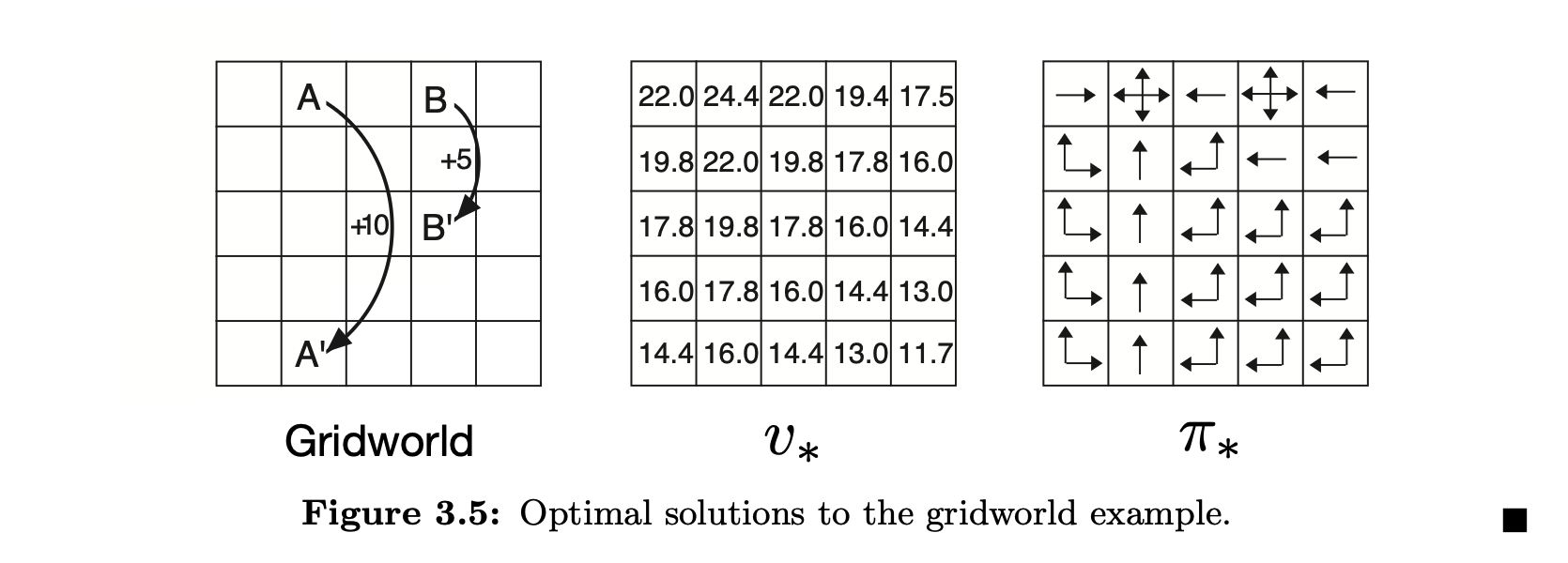
When someone says optimal, then the next question should be optimal with respect to what? Since none of the other squares have any reward, to make sure we move towards a point where we get rewards we need to think of eventual rewards. However we also want the player to favour immediate rewards over possible rewards at a later point in time. That's pretty much the crux of the problem all Reinforcement Learning problems try to solve. The reward we get 10 steps down the way is worth less than the reward we get right away. So we discount the reward we could get after one time step by a factor of $ 0 < \beta < 1$. This discount factor determines the behavior of the player, if we don't discount it enough every move will gravitate toward $0,1$, if $\beta = 0$ it's basically move randomly. We can calculate the discounted reward for each position like

We just find the reward at next step and discount it by $\beta$ for this iteration, if it's not a wormhole or outside the bounds. But how do we find the reward for the next step? This feels recursive, but also fits beautifully into our pattern of finding fixpoints. This specific equation form is called Bellman optimality condition. And this is also an equilibrium point. But won't this explode to infinity? Fortunately no. This always has a bounded solution provided $C$ is bounded (has a maximal value). This form of discounted functions is often used to evaluate infinite cash streams, like bonds. Will leave the code for this one out, the discount factor used for the image above is $\beta = 0.9$

Expectation Maximization

Here we use the simplest example used by Chuong B Do & Serafim Batzoglou in What is Expectation Maximization?. Suppose you have two biased coins (not 50-50 chance), and we pick one coin at a time and toss it 5 times and record whether it's head or tail. And we repeat this 5 toss experiment, let's say 10 times. We have a total of 50 tosses/samples, and now we want to estimate the bias of the two coins we used. We don't know which of the 10 experiments used which of the coins. This is where the Expectation Maximization algorithm comes in.

It follows our by now familiar structure, we guess the bias and find which of the coins could have most likely produced the output. Assuming the most likely coin, we re-estimate the biases. Rinse repeat. To rephrase let's assume we have a function $f$ that takes current bias estimates $(\theta_1, \theta_2)$, assigns experiments to most likely coins, re-estimates biases, and returns new $(\theta_1', \theta_2')$. We can repeatedly apply $f$ to the revised estimates until .... it reaches a fixpoint/convergence where it stops changing.

                    
MAX_ITERATIONS=100
EPSILON = 0.01
import random
toss_per_experiment = 5
num_experiments = 10


def experiment(theta_1, theta_2):
    chosen = [theta_1, theta_2][random.randint(0, 1)]
    return random.binomialvariate(n=toss_per_experiment, p=chosen)

# What's the probability this experiment is produced with this biased
# for the coin
def expectation(num_heads, theta):
    prob_heads = theta ** num_heads
    prob_tails = (1 - theta) ** (toss_per_experiment - num_heads)
    return prob_heads * prob_tails
    

def em_bias(experiments):
    theta_1, theta_2 = 0.4, 0.6
    num_iterations = 0

    while num_iterations < MAX_ITERATIONS:
        # Number of heads in experiments assigned to this coin
        sum_ex_1, sum_ex_2 = 0, 0 

        # Total Number of coin flips in experiments assigned to this coin
        count_ex_1, count_ex_2 = 0, 0 
        for num_heads in experiments:
            e1 = expectation(num_heads, theta_1)
            e2 = expectation(num_heads, theta_2)
            if e1 > e2:
                sum_ex_1 += num_heads
                count_ex_1 += toss_per_experiment
            else:
                sum_ex_2 += num_heads
                count_ex_2 += toss_per_experiment
        next_1, next_2 = sum_ex_1 / count_ex_1, sum_ex_2 / count_ex_2

        if abs(theta_1 - next_1) < EPSILON and abs(theta_2 - next_2) < EPSILON:
            break

        theta_1, theta_2 = next_1, next_2

        num_iterations += 1
    
    return theta_1, theta_2

# This gets close, and closer as we increase 
# - the number of toss "and" 
# - the number of experiments
em_bias([experiment(0.4, 0.8) for i in range(num_experiments)])
                    
                

Note the above code does what is called Hard Expectation Maximization, whereas what the paper referred to does Soft Expectation Maximization. The Soft/Pure version is a bit more sophisticated and uses Bayes theorem to estimate the next iteration $\theta$. This is far simpler to explain the theme of the story without digressing a lot into Bayesian estimations. However even soft version fits into the same framework.

This example however feels like a very cooked-up scenario, not very easy to see how anyone could use this in practice to solve real problems. The following example illustrates how such an estimation with incomplete information is useful. Suppose you are given a corpus of pairs of sentences in say English and French, you need to build a dictionary of word pairs. How do you go about doing that? Both the languages could have different word orderings, so the same word could appear at different positions (attention heatmaps in transformer models could point to this). There is also this problem of synonyms, being used for different sentences. And a single word could be mapped into a multiword phrase and vice-versa. It all feels very fuzzy, until we lean on our framework of thinking through such problems.

First in order to accommodate the multi phrase mappings, synonym structure and also to make the EM algorithm more robust we do soft pairings, we don't say the French word $le$ means $the$, but instead assign a probability to that pairing. Next we build a function using those soft probabilities, we can estimate how likely the sentence pair alignment is, then adjust the soft pairing probabilities, until we reach a fixpoint where the soft pairings get stable. That's a very short and crude version of how IBM solved the machine translation using EM algorithm described in Brown, P. F., Della Pietra, V. J., Della Pietra, S. A., & Mercer, R. L. (1993). "The Mathematics of Statistical Machine Translation: Parameter Estimation."

Got a hammer - everything is a nail

In Structure and Interpretation of Computer Programs, the first chapter opens with the problem of finding square root. They use Newton Raphson method to find the roots/solution to the equation $f(x) - a = 0$ where $f(x) = x^2$. The Newton iteration simply iterates over

On a closing note, fixpoints are truly versatile. They appear a lot in computability theory too, for example, there is a theorem proved by Kleene about how every total computable function admits a fixpoint, which I learnt about from this nice little puzzle book called To Mock a Mockingbird by Smullyan. Smullyan has a brilliant mind to elegantly put a lot of combinatorial logic as birds chirping to each other. I definitely recommend that book.

Speaking of books, I definitely recommend one other book which absolutely blew my mind, where I got the first introduction to Banach fixpoint theorem, Conceptual Mathematics: A First Introduction to Categories by Lawvere and Schanuel. Brilliantly written, very very approachable to noobs like me.