Computing, Math and Beauty

What is information?

The first time I visited Amsterdam, it was in April. Having lived only in tropical regions for my entire life by then, I was surprised (or perplexed) to find the sun at 9:00 PM (Central European Summer Time). I have learned about long days, but never really thought that 9:00 PM could be so bright. This was new information to me. This qualitatively has more information than, let's say, the sun rising in the east. The goal of this post is to build a framework to reason about this qualitative feeling and give it a solid grounding to objectively measure and talk about what we intuitively know as information.

What the above story illustrates is that the information is associated with events. And somehow if an event I didn't expect happens then there is more information in the event than the one I expect did happen. So the information content in an event is related to the probability of the event. Given an unbiased coin (50-50 chance of head or tail), let's assume that the event that a single toss of the coin results in heads (probability 0.5) has information of 1 unit. Why should this be 1? Because we choose it to be, also because it's the simplest probabilistic event we can think of. Given we established that, intuitively we can also say, two coin tosses, both resulting in head have double the information of a single toss resulting in head (since it's rarer). Independent events multiply probabilities, but the information of independent events should add. This multiplication turning into addition is the first clue towards finding a function $I$ which, given a probability of an event, gives the information content in the event, from what we know for now.

Let's represent pictorially the multiple coin toss experiment as follows. Each node represents an event of $k$ tosses at depth $k$, let $N_k$ be the number of nodes at level $k$. The probability of any event represented by the node at depth $k$ is represented as $p_k$. And $p_k = \frac{1}{N_k}$ (uniform probability, we assumed unbiased coin) and therefore $N_k = 1/p_k$.

The information content in each node is equal to the depth at which the node is present. $I(node) = depth(node) = k$

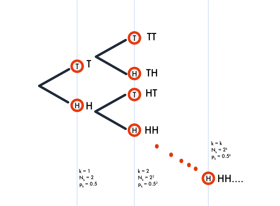
As every programmer knows, the number of nodes at level $k$ of a complete binary tree, ie., $N_k$ is $2^k$ and therefore $\operatorname{log}_2{N_k} = k$. It is also intuitively clear from our previous argument each individual event represented as a node has an information content equal to the depth $k$ (depth $k$ means $k$ tosses, we established one coin toss is 1 unit of information). Since $N_k = 2^k$ and $p_k = \frac{1}{N_k}$, we can say $I(p) = k = log_2(2^k) = log_2(1/p) = - log_2(p)$.

Thus we have derived what information means from first principles and how it relates to probability. It would also be clear why the unit of information is a bit (take head as $1$ and tail as $0$, we have one bit introduced per toss). However note that this notion of bit is no longer a positive integer but a positive real number, suppose we have some event that occurs with a probability of $1/\sqrt{2}$ the amount of information in it is $0.5$ bits. At the end of this post we should be able to shake off this uneasy feeling towards dealing with non-integral bits.

Expected length

Usually timeseries like stock prices (or even videos) are encoded (turned into bit representations) using something called Delta encoding. We generally won't send the stock price as such, we instead send only the difference, like +0.05, -0.25, 0.0 etc., after the initial value. The receiving side would cumulatively add them to reconstruct the timeseries back. Since the stock prices don't change a lot, these differences would be very small. The idea is to encode smaller values with fewer bits vs larger number with more bits. The usual fixed number of bits encoding of floating point values adds no advantage with differential encoding. To generalize this notion even further, we need to encode more probable values with fewer bits compared to less probable ones.

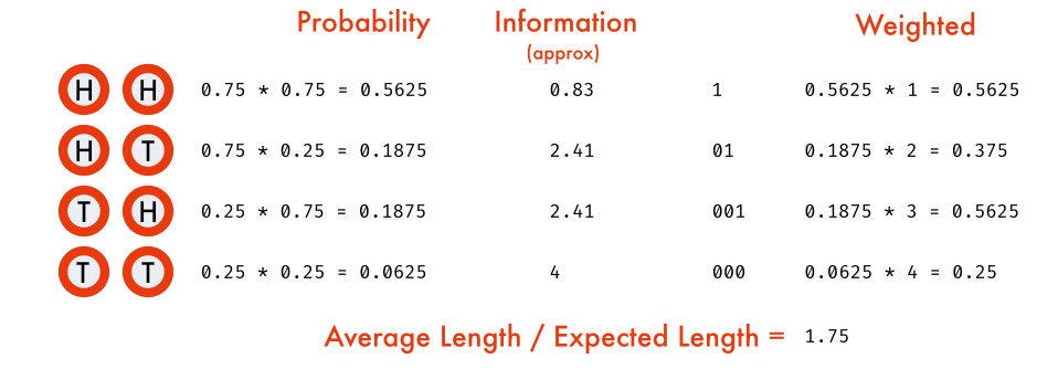
Consider this simpler scenario, we have a biased coin which results in head with $0.75$ probability and tail with probability of $0.25$, we need to send (or store) the outcomes of $n$ tosses of the coins. It's grossly inefficient to store head as $1$ and tail as $0$. As the resulting sequence would be predominantly $1$ (more probable). Since information content is inversely proportional to the probability of the event, what if we define an encoding where we assign information number of bits for each outcome to encode it? (another reason why unit of information is called bits). But the problem as we saw earlier was information could be fractional/real. In this case $I(H) \simeq 0.415$ and $I(T) \simeq 2$. We can easily encode tails with 2 bits, but head? How can we have 0.415 of a bit?

The trick is to encode them as blocks. Let's take two coin tosses at a time.

If we take two coin tosses at a time and encode it in the order of probability. Average number of bits to encode 2 coin tosses is already smaller ($1.75 \lt 2$). This approaches the optimal bit length from information, longer the sequence becomes. Note that we made sure that prefixes are uniquely decodable, if we could encode it we should be able to decode it properly.

In a similar fashion, the timeseries with delta encoding can also be compressed by taking a distribution that represents the population as close as possible, since the differences are usually small and close to 0. A normal distribution would work wonders (with mean = 0 and std-deviation calculated from the general volatility). There are a few tricks to discretize a continuous distribution like binning etc.. The general idea is we can use information as a guide to encode the sequences efficiently.

Entropy

We came across this notion of expected bits required to encode an event, by doing weighted average of information with the probability (like any expectation is), this is called Entropy. It is usually denoted by $H(P)$ for a probability distribution $P$. We just sum over all the outcomes the product of information of the outcome (bits required) with its probability.

Entropy signifies the general compressibility of a data source. The uniform distribution is absolutely incompressible. But any distribution where one thing can happen more than another, we can exploit that. Entropy is the measure of how skewed such distribution is. The more skewed the data source, the more compressible it is. Entropy is the north star for compressibility of a data source.

For example let's take an event with four outcomes $\{A, B, C, D\}$ with probability $P = (0.5, 0.25, 0.125, 0.125)$ respectively. The individual information in each event is $(1, 2, 3, 3)$.

                    
import math

def information(prob):
    return - math.log(prob)/math.log(2)

def entropy(outcomes, prob):
    return sum(prob[outcome] * information(prob[outcome]) for outcome in outcomes)
    
                    
                

Cross Entropy and KL divergence

A lot of the time, when we work with a stochastic process, we won't know the exact probability distribution, either because the population is too large or it is difficult to model the exact process. In such cases we take a different probability distribution, usually estimated from a much smaller sample or a much simpler process. Now if we try to encode the sequences generated by the original process, but encoding assigned based on our approximate probability distribution, our expected bit length would be different from entropy.

This entropy calculated from two different distributions one to encode and the other to produce expectation is called Cross Entropy (denoted by $H(P, Q)$). The distribution $P$ is the process by which the data is produced, but since we don't know that we use $Q$ to decide how many bits each outcome should take. And somehow we are able to achieve the limit imposed by $Q$ (fractional bits and block encoding), then cross entropy calculates the amortized cost or bits required per outcome.

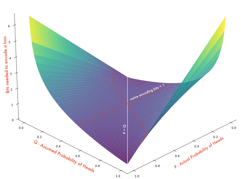
Note that, the cross entropy becomes entropy when $P = Q$. In fact, $H(P, Q) \ge H(P)$ (Gibbs' inequality). To illustrate, let's take our previous experiment of the biased coin toss with $P$ as probability of heads. And we didn't know $P$ and we assumed $Q$ to be the bias of the coin ie., the probability at which the coin turns head is $P$ but we didn't know that and we assumed it to be $Q$. The following chart shows the plot of $P \in (0, 1)$, $Q \in (0, 1)$ vs its cross entropy $H(P, Q)$.

Plot of biased coin with probability $P$ for head which we don't know and $Q$ is our guess with their Cross Entropy $H(P, Q)$. The valley is at the line where $P = Q$. Also note the naive encoding contour lines (red), $z = 1$ crosses the line $P = Q = 0.5$. This shows, that in uniform distribution, naive encoding is as good as it gets.

The cross entropy, especially binary cross entropy (coin toss - Bernoulli distribution), is used a lot as loss/objective function in the gradient descent of deep neural networks. Cross entropy (multi targets) is the loss function used in all LLMs for example. In LLM training, every training label (next token, in auto regressive models) is assumed to have $P = 1$ ($P$ is one hot, ie., $1$ for correct token and $0$ for others) and $Q$ is what we predicted the probability of that particular token is (usually softmax). Thus reducing the loss to just $-log_2(Q)$ for correct token (next token dictated by the data point we are training now) and it vanishes for wrong token as $P = 0$ for incorrect tokens.

In the example we used in the Entropy section, for four outcomes $(A, B, C, D)$ with probability $P = (0.5, 0.25, 0.125, 0.125)$ suppose we somehow mistook $A$ for $B$ while estimating and used resultant $Q = (0.25, 0.5, 0.125, 0.125)$ as our encoding distribution, then the cross entropy is

The difference between the cross entropy and the entropy (wastage of not knowing the actual probability distribution) ie., opportunity cost or wastage we incurred above, is called Kullback-Leibler (KL) divergence. It is the difference in the number of bits required in our flawed encoding vs the optimal encoding as dictated by the probability distribution. In the above example it is $H(P, Q) - H(P) = 2 - 1.75 = 0.25$. Cross entropy and KL divergence form the same loss surface (one is monotone transformation of other). $D_{KL}$ differs from $H(P,Q)$ by a constant $H(P)$ as the probability distribution $P$ is fixed. So as loss function either is replaceable by the other. KL divergence is expressed in any of these forms,

Mutual Information

Suppose we have two events, the lawn is wet $W$ and it rained today $R$ (very cliched example, I know). If lawn is wet, the chances that it rained today are very substantial. We express this using conditional probability $P(R|W)$. But we aren't interested in that. How much information would the event that it rained today have before we find the lawn wet and after we find the lawn wet? They should be different. Intuitively, lawn being wet has some information about rain earlier today. The difference between the information I would have gained from the fact that it rained today before and after knowing the lawn is wet, is called Mutual information.

To put it concretely how much information one event gives about other is called Mutual information. Given two random variables (think of it as just functions from outcomes to a real number, there is some technicality on what kind of functions can be a random variable, but only really weird ones aren't.) $X$ and $Y$ we can find the entropy $H(X)$, which gives the expected information on $X$. We could also find $H(X|Y)$ which gives the information on $X$ given $Y$ has occurred (swap the probability distribution with conditional probability distribution). The occurrence of $Y$ could increase or decrease the odds of $X$ and thereby decrease or increase the information respectively on $X$ happening. This kind of gives us a notion of how much information one has over other. For independent events, they obviously would be $0$. Thus putting that into formula

In the above example if $P(R|W) = 0.75$ and $P(R) = 0.25$ then, originally had we learnt the fact that it rained before finding the lawn wet we would have had $I(R) = 2$ now after finding out it's wet, $I(R|W) = 0.415$ and the mutual information gives us the information that lawn being wet provides over rain $I(R; W) = 1.585$. This is just *Point wise Mutual information*. It's a single event analogue of Mutual Information. PMI is to Mutual Information, what Information is to Entropy. Mutual information is defined for the complete distribution, for that we need to find the entropy of the entire distribution. Will leave it here, as that's just technical complication and adds no real understanding from working it out. Note that, this notion of Mutual information is symmetric unlike cross entropy or KL divergence. This could be inferred very easily from Bayes theorem (leaving that out as exercise too).

Some more..

Another measure that's very popular these days is Perplexity. Given a probability distribution, we are trying to find how many equiprobable outcomes we could get with the same entropy. More intuitively, if we were to design an unbiased die which had same entropy as given probability distribution, how many sides (possibly fractional) should it have. It's like a notion of normal form or equivalence classes of entropy. Put it differently, if we were to establish our bits into a tree like above (imagine fractional branches), how many leaf nodes would be there? That kind of tells us how many different equiprobable outcomes we can expect from a distribution. For example, if we have a biased die with entropy $H(D) = 2$ that's equivalent to an unbiased $2^H = 2^2 = 4$ sided die (imagine), as far as entropy is concerned.

This notion is used in LLMs to measure how surprised the model is on a text ie., If a model produced a text sequence $S$ with probability $0.5$ that only adds as much information as a coin toss. It gives us a way to compare information content between models. In LLMs we are comparing a given text sequence with the corpus distribution the LLM model is trying to mimic. It's sort of estimating the luck of generating a text compared to "perplexity" sided die given a model.

Information theoretic view is about interpreting everything through this number of bits lens. It should be easier now to understand why zipping a zip file won't do much, for example. If we start using it a lot we find this lens to be very powerful, it could explain everything from intelligence to physics. There are a lot of new attempts to reframe some of the fundamental physical systems (thermodynamics to black hole information) through information theory. Intelligence for example can be interpreted as compressing the information we gained using the patterns we acquired. We don't remember everything we learn, some of which we derive on the fly from first principles. What we call intelligence is just compression. And it helps us distinguish intelligent beings/things from those that are not so much (it's a spectrum I suppose). We could probably build a more robust version of Turing test based on information theory and compressibility too. Once we learn to see through this lens, we can easily come to the conclusion that, information is more fundamental than it seems.