Polynomial fit: a rabbit hole

15 Jun 2026

I started working on a small project of trying to compress timeseries within a given bit (or byte) budget. The library would allow one to compose various primitives and it would choose the combination that compresses the timeseries within the budget minimizing the mean squared error. The primitives could be polynomial, fourier series, simple8b (I have a modification by quantizing the floating point value by choosing the bits for a given budget) and the algorithm would recursively try to fit the residuals to improve the accuracy by splitting the budget. One can think of it as finding a point of interest in Pareto Front of budget and accuracy.

The polynomial fit is the one I grossly underestimated. I thought if I treat each of $x, x^2, x^3...$ as independent variables then I can just do ordinary least squares (linear regression) and be done with it. I realised it's not as simple as I thought. And the solutions I found rephrase the problem so beautifully that I had to write about it.

Vandermonde Matrix

If we were to express the polynomial fit as a linear regression problem, $Xa = y$, where $a$ is the coefficients we are fitting, then $X$ has the form,

$$ \begin{bmatrix} 1 & x_1 & x_1^2 .... & x_1^n \\ 1 & x_2 & x_2^2 .... & x_2^n \\ 1 & x_3 & x_3^2 .... & x_3^n \\ ... \\ 1 & x_m & x_m^2 .... & x_m^n \\ \end{bmatrix} $$

Obviously, we are trying to express the powers of $x$ as independent variables here. This particular matrix is called Vandermonde matrix. There are few issues with this formulation of polynomial fit arising from both the structure of the problem defined this way and how representable floating point numbers are distributed in its domain.

Distance between successive floating point numbers varies across representable range. It is densest close to 0 and sparser outward.
Img Credit: Wikimedia

Floating point doesn't have infinite precision and it doesn't even have equal precision everywhere. Suppose $|x| > 1$, then $x^n$ would be so large that there is very little accuracy if it is representable at all. Similarly if $|x| < 1$ then $x^n$ would be too small and you hit the opposite problem. So any representable Vandermonde matrix for sufficiently large $n$ is error prone in one way or another. Also even if we manage to fit accurately, the coefficients would have opposite problems of the factors (smaller $x$ implies we need larger $a$ to make it matter and vice versa) and hence inaccuracies in how the coefficients are represented.

Some part of this problem is also captured through this notion of Condition number of a matrix, which is the product of the norms of matrix and its inverse. Condition number specifies how small errors in $y$ affect $a$. This sort of measures how stable our solution could be to small errors or perturbation in $y$. Vandermonde matrix has very high condition number. So this way of fitting is unstable for all but very small $n$.

Geometry and Orthogonality

While posing the polynomial fit as linear regression we chose the representation of the function to be a vector in coefficient space. The standard basis here is assumed to be the monomials $1, x, x^2 ....$. And since this is the standard basis they are clearly orthonormal by the choice of representation. We need to distinguish this space from another space which we are really interested in, so let's call this space coefficient space of the polynomial.

What we are actually interested in is the function space, not the coefficient space. We want to talk about the functions, or just polynomials, without talking about their representation. This is more of an extensional notion of a function, defined purely by the values it takes at each point in its domain. In general that domain is continuous and the space is infinite dimensional. Our extensional notion wouldn't care whether the function is transcendental like $\sin$, $\cos$ and $e^x$. For curve fitting we only look at finitely many sample points, so it stays discrete and finite. This space should have an inner product or dot product structure (we call two functions orthogonal when their dot product is zero), and that inner product should also be defined extensionally, from the values alone, without worrying about how the function is represented. Let $f, g$ be two functions defined on the same set of discrete points $x_i$, we define inner product $$ \langle f, g\rangle = \sum_{i} f(x_i)g(x_i) $$ Note that this has no notion of representation built into it. It's totally based on what values either function takes on each of the values in input domain. This also synergizes with our objective of minimizing sum squared loss, since the points are $y$ values the function takes for a pre-chosen set of $x$s.

To be clear, we have two geometries at play here,

Coefficient space - Representing polynomial as coefficient vector by assuming that monomials $\{1, x, x^2...\}$ are an orthogonal basis. And inner product between two functions (here represented by a vector) is just sum of product of the coefficients.
Function space - Representing polynomial by the value it takes. The orthogonality just bubbles up to you, we didn't force orthogonality. It totally depends on function and is invariant to its representation.

For example: Lets take $x = [0, 0.1, 0.5, 1]$ and $x^2 = [0, 0.01, 0.25, 1]$, these two taken in coefficient space ($f = [0,1,0]$ and $g = [0, 0, 1]$) are orthogonal because we took the standard monomials as basis. But in function space we can find the angle between them using cosine form of the inner product.

$$ \begin{align} \cos(\theta) & = \frac{\langle f, g \rangle}{|f||g|} \\ & = \frac{0 \times 0 + 0.1 \times 0.01 + 0.5 \times 0.25 + 1 \times 1}{(\sqrt{0 \times 0 + 0.1 \times 0.1 + 0.5 \times 0.5 + 1 \times 1})(\sqrt{0 \times 0 + 0.01 \times 0.01 + 0.25 \times 0.25 + 1 \times 1})} \\ & \approx \frac{1.126}{1.123 \times 1.031} \\ & \approx 0.973 \end{align} $$

Above calculations are just mostly elementary bookkeeping, but the result is enlightening as $\cos^{-1}(0.973) \approx 13.3^\circ$, that's nowhere close to being orthogonal. They are in fact more parallel than orthogonal (but clearly independent). Intuitively, the reason for large coefficients (in absolute terms) is that each higher order coefficient enters into competition on who matters and tries to cancel each other out. Particularly as shown in the picture, if the basis vectors are close to being parallel in one direction, to represent any vector that has considerable component in the orthogonal direction, it takes long detours. This large distance travelled in parallel directions needs to be cancelled out by each other. It pinpoints the root cause of lack of algorithmic stability in polynomial fit using standard monomial basis, that they are not orthogonal in the space that matters, the function space.

$f$ is short, but $a$ and $b$ are both large and opposite in sign. Because $x$ and $x^2$ are nearly parallel, representing anything that points away from them needs big cancelling coefficients, and that cancellation is where floating-point precision dies.

Forsythe Polynomials

George E. Forsythe in 1957 wrote his paper Generation and Use of Orthogonal Polynomials for Data-Fitting with a Digital Computer. In it he described how to find a good orthogonal set of polynomials. The least square fit just comes out naturally from linear algebra through projection. Section 6.61 of Linear Algebra Done Right by Sheldon Axler states this cleanly. The vector in a subspace (in our case subspace being polynomial of certain degree) at the shortest distance from a given vector is just the orthogonal projection of that vector onto the subspace. Here the vector being projected is our extensionally defined function, and the subspace is spanned by the orthogonal polynomials we build up to some fixed degree. Axler shows a similar example in that section, approximating $\sin$ by a polynomial. At its core we are doing the same thing. It's beautiful how the problem crumbles into a solution when we choose the right abstraction.

Forsythe describes a family of orthogonal polynomials, using a recurrence. Which goes like this,

$$ \begin{align} P_0(x) & = 1 \\ P_{n+1}(x) & = (x - \alpha_n)P_n(x) - \beta_n P_{n - 1}(x) \end{align} $$

Though the polynomial recurrence looks arbitrary, we could have discovered them from first principles. What we need is a family of polynomials $P_n$ which are orthogonal to each other. Note we also would like the fact that $n$^th polynomial has the degree $n$ (This has nice consequences, they are called graded polynomials and let us preserve subspace containment if we switch to a different basis which is also graded, we need this later). Now simplest polynomial we can build of degree $n + 1$ is just $xP_n(x)$. Thus we have a polynomial of degree $n+1$ we just do one step of Gram-Schmidt orthogonalization (fancy name for subtracting away projection of other $n-1$ polynomials we built). Thus,

$$ \begin{align} P_{n + 1}(x) & = xP_n(x) - \sum_{i = 0}^{n} \frac{\langle xP_n(x), P_i(x) \rangle}{\langle P_i(x), P_i(x) \rangle} P_i(x) \\ & = xP_n(x) - \sum_{i = 0}^{n} \frac{\langle P_n(x), xP_i(x) \rangle}{\langle P_i(x), P_i(x) \rangle} P_i(x) \end{align} $$

There are two things happening here

We used the fact $\langle x P_n(x), P_i(x) \rangle = \sum_j x_j P_n(x_j) P_i(x_j) = \langle P_n(x), x P_i(x) \rangle$. This can also be understood from another angle, that $xP_n(x)$ is doing a Hadamard product. And Hadamard product can be expressed as a diagonal matrix, which is self adjoint (it is its own transpose) and hence can move between the terms in inner product.
$xP_i(x)$ has degree $i+1$, so it is a linear combination of $P_0, \dots, P_{i+1}$. Since $P_n$ is orthogonal to every polynomial of degree less than $n$, the inner product $\langle P_n, xP_i\rangle$ vanishes unless $P_n$ shows up in that combination, which needs $i+1 \ge n$. So only $i = n-1$ and $i = n$ survive, because $xP_{n-1}$ has degree $n$ and $xP_n$ has degree $n+1$.

This leaves only two of the terms in the summation. Thus we can simplify the above equation as,

$$ \begin{align} P_{n+1}(x) & = xP_n(x) - \frac{\langle P_{n}, xP_{n} \rangle}{\langle P_{n}, P_{n} \rangle} P_n(x) - \frac{\langle P_{n}, xP_{n-1} \rangle}{\langle P_{n-1}, P_{n-1} \rangle} P_{n-1}(x) \\ & = (x - \alpha_n) P_n(x) - \beta_n P_{n-1}(x) \end{align} $$

Which has the familiar form of Forsythe recurrence, where,

$$ \begin{align} \alpha_n &= \frac{\langle P_{n}, xP_{n} \rangle}{\langle P_{n}, P_{n} \rangle} &= \frac{\sum_i x_i P_n(x_i)^2}{\sum_i P_n(x_i)^2} \\ \beta_n &= \frac{\langle P_{n}, xP_{n-1} \rangle}{\langle P_{n-1}, P_{n-1} \rangle} & = \frac{\sum_i x_i P_n(x_i) P_{n-1}(x_i)}{\sum_i P_{n-1}(x_i)^2} \\ \end{align} $$

Note that the polynomials totally depend only on $x_i$ if we squint our eyes a bit, it looks more like neural network pre-training (except there is no compression, the dimension remains the same). Find a representation which naturally represents our input. Once we have the polynomials, we can find the coefficients again by projecting our $y$ onto each of the polynomials $P_{n}$ (dot product and rescale it) thus derived. This satisfies our objective of minimal sum squares due to our choice of inner product, for free.

Chebyshev polynomials

For the timeseries compression use case, I condition the input further by scaling $x$ (or $t$ whichever independent variable is preferable) into $(t - mid)/mid$ to keep it within well represented bounds of floating point ie., $[-1, 1]$. The $x$ values I have are equidistant from adjacent elements and more importantly completely derivable from just a single number, the total number of points $n$. I just need to store that along with the Forsythe's polynomial and I can reconstruct the polynomial on the fly. Since the recurrence is very stable (we are multiplying by readjusted $x$ value one step at a time), I can use that to predict the $y$ value for each of my $x$. To be clear there is no reason for me to store the Forsythe's polynomials, ie., $\alpha_i$ and $\beta_i$. All I need to store is $k$ coefficients along with $n$, so $k+1$ numbers.

Unfortunately, not everyone doing polynomial fit has the luxury of such well behaved independent variable domain that they can get away with not storing them. To reconstruct the polynomials they need $3k$ numbers ($\alpha_i$, $\beta_i$ and coefficients). We could collapse the Forsythe polynomials into monomial form to avoid storing $3k$ numbers, but that drops us right back to square one of numerical instability. If only we had a standard set of orthogonal polynomials independent of our data which also form a well-conditioned graded basis, we could use that and just store $k$ values instead of $3k$. And fortunately Chebyshev's polynomials are exactly that.

Chebyshev also defines a family of orthogonal polynomials as,

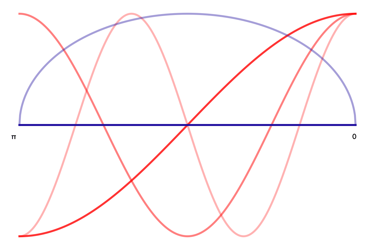
$$ T_n(\cos(\theta)) = \cos(n\theta) $$ or $$ T_n(x) = \cos(n \cos^{-1}(x)) $$

How is that a polynomial? It is intuitive once we find out that $\cos(n\theta)$ is a polynomial in $\cos(\theta)$ (apply trigonometric formula for $\cos(a + b)$). What Chebyshev did was to transform the $[-1, 1]$ into $\cos$ space in $[0, \pi]$, like put in an interpreter in between to translate $x$ into something where $\cos(n\theta)$ could be treated as a polynomial. Polynomial form can also be seen by deriving a recurrence relation. It just needs some trigonometric manipulation using $\cos(a+b)$ expansion. Also observe we don't have discrete set of points to find the inner product, Chebyshev integrates (instead of summation) over the entire domain $[-1, 1]$ and the inner product is scaled to take care of deformation caused by pretransforming $x$ by $\cos(\theta)$, the Jacobian of the change of variables.

$$ \langle f, g \rangle = \int_{-1}^{1} \frac{f(x)g(x)}{\sqrt{1 - x^2}}dx $$

What looks like transcendental function in $\theta$ space starts to look like polynomials in $x \in [-1, 1]$ after $\cos^{-1}$ transformation. That's Chebyshev's insight. We are distorting the x-axis into top of a unit circle (it is centered here).

Clenshaw's algorithm

Given that Chebyshev gives us a more data-independent orthogonality we could represent our polynomials as coefficients of that basis. Why not fit directly onto Chebyshev basis? If we look carefully there are two approaches to doing that, but both of them fall flat on our motivation,

The terms of the basis look like the real part of a Fourier series. Ideally we could fit using FFT which might in fact be the fastest and numerically stable method in this case. But FFT requires the sample points to reside at the Chebyshev extreme points (peaks and troughs of the $\cos n\theta$). it would work well if the sample points are uniformly spaced in $[0, \pi]$. It won't work even in my timeseries compression case, as instead of uniformly spacing in $[-1, 1]$ I would have to uniformly space it in $[0, \pi]$ at that point it is a Fourier transform. It captures periodicity like Fourier does but not the inherent polynomial structure my data might have.
We cannot use the projection theorem on Chebyshev basis like projecting our points onto its basis because it would no longer be a normal least squares fit. Because the inner product is not discrete sum on our data points and moreover its scaled by Jacobian. Chebyshev polynomials are orthogonal in a different $\cos$ distorted space, the direct projection would possibly be $\cos$ weighted least squares having least weights on points closer to $0$ and diverges to $\infty$ on either end. There might be use cases for it where we care more about accuracy at the start and end (stock prices?) than at the middle. However I don't think we need classism in how each $x$ value is treated unnecessarily.

If we need proper least squares result on Chebyshev basis, then we need to transform the Vandermonde matrix (without building it explicitly, once you build it, your garden is full of weeds) into Chebyshev basis. It is better conditioned than the monomials, so solving it is stable. But they aren't orthogonal at your sample points, we need full least squares solve through normal equations. Forsythe is orthogonal at your data points like how PCA adapts to your data points, and hence just the projection on subspace theorem works.

But Clenshaw in his paper Curve fitting with a digital computer, addresses the memory issue and the conditioning issue. He came up with a clever idea. He proposed we fit the polynomial using Forsythe's recurrence and then turn the basis into Chebyshev's. Now we could get away with not storing $3k$ values and store only $k$ coefficients of Chebyshev's polynomial. Since it is standard, we could prebuild the polynomials during inference/interpolation time and could ideally reconstruct the polynomials. But that's not his only contribution in that paper, he gave a nicer more numerically stable algorithm to evaluate the polynomial at individual points. The algorithm has nothing Chebyshev-specific, it just needs the series to follow a definite recurrence structure,

$$ \Phi_{k+1}(x) = \alpha_k(x) \Phi_{k}(x) + \beta_k(x) \Phi_{k-1}(x) $$

Note that this could work even for Forsythe structure we had (form is immediately clear). If there is a single take away from this post it is this, a stable recurrence is one of the most beautiful ways to turn an algorithm into numerically stable one. You keep weeding out problems every step and it always stays in well represented space at each iteration. Sort of like how we would like to keep the gradient norm to be close to $1$ between layers of neural networks.

As Gilbert Strang once said, you can never learn enough linear algebra. There is always something new that you have never seen. This notion of filtration and graded polynomials is something I learnt on the way. Writing them down was a fruitful exercise. It helped me be absolutely clear on what I might have generally hand-waved. It gave me great insights that I might have missed. I suppose now I believe Writing to Learn. Why bother, in an age where the AI does it for you? Partly so you can tell when the AI is bluffing. And partly because some things are just worth collecting for their own sake, which is what I earned by beating my head against this for over a week, when I could have thrown a library at it and been done.